flowchart LR
  A["DICOM"] -->|dcm2niix| B["NIfTI"]
  B --> C["Draw ROIs<br/>(3D Slicer / ITK-SNAP)<br/>gastrocnemius, soleus, tibialis anterior"]
  B --> D["Compute quantitative maps<br/>(Python)<br/>T2, fat fraction, TSC"]
  C --> E["Mean values and volume within ROI"]
  D --> E
  E --> F["Statistical analysis<br/>(R / Python)"]
8 Quantitative Analysis and Software
8.1 Data formats
| Format | Contents | Main use |
|---|---|---|
| DICOM (.dcm) | One file per slice. Image plus tags for acquisition parameters (TR, TE, pixel size, patient information, etc.) | Original data from the scanner; hospital imaging systems |
| NIfTI (.nii / .nii.gz) | A 3D or 4D image in one file, with the mapping between pixels and space (orientation, pixel size) | Standard for research analysis software |
| Scanner raw data (Siemens .dat, etc.) | k-space data | Custom reconstruction (e.g., 23Na UTE) |
dcm2niix (command line, bundled with MRIcroGL) is commonly used to convert DICOM to NIfTI.
WarningWatch out for personal information
DICOM tags may contain names, dates of birth, IDs, and so on. Always anonymize the data (delete or replace tags) before sharing it for research.
8.2 Commonly used software
| Purpose | Software | In short |
|---|---|---|
| Viewing images, drawing ROIs | 3D Slicer (Fedorov et al. 2012) | Free and feature-rich. Segmentation, volume calculation, many plugins |
| Semi-automatic segmentation | ITK-SNAP (Yushkevich et al. 2006) | Handy for painting muscle and fat regions. Also used for ROI creation in a skeletal muscle 23Na study (Höger et al. 2023) |
| Viewing DICOM (Mac) | Horos / OsiriX | Viewers widely used in hospitals and clinical research |
| Brain image analysis | FSL (Jenkinson et al. 2012), FreeSurfer, SPM, ANTs | Registration, brain segmentation, etc. Sometimes also used for registration in muscle research |
| MRS analysis | LCModel, jMRUI, OXSA (MATLAB, 31P), FSL-MRS | Fit peaks to spectra to quantify metabolites |
| Numerical computing, custom analysis | Python (numpy, scipy, nibabel, pydicom, SimpleITK, scikit-image), MATLAB, R | Map calculation, statistics, figures |
| Bundled with the scanner | syngo.via (Siemens), etc. | Clinical reading and measurement |
8.3 A typical analysis workflow (calf muscle example)
TipTips for drawing ROIs
- Avoid fascia, large vessels, and bone boundaries, and draw inside the muscle (to avoid partial volume effects) (Höger et al. 2023)
- For low-resolution images such as 23Na, draw ROIs on high-resolution 1H images and then overlay them on the 23Na images (Höger et al. 2023)
- Take steps such as marking the skin before scanning so that the slice position is the same every time
8.4 Python 1: make a T2 map
From 16-echo images with different TEs (synthetic), we fit \(S(TE) = S_0 e^{-TE/T_2}\) pixel by pixel. We compute it in two ways: first taking the logarithm and fitting a straight line (fast), then nonlinear fitting (accurate).
code/08_t2map.py
# Create a pixel-wise T2 map from multi-echo images (synthetic)
import numpy as np
import matplotlib.pyplot as plt
from scipy.optimize import curve_fit

rng = np.random.default_rng(2)
N = 64
y, x = np.mgrid[-1:1:N * 1j, -1:1:N * 1j]
leg = x ** 2 + y ** 2 < 0.85 ** 2

# true T2 map: muscle 40 ms, edema in the upper right (T2 = 60 ms)
T2_true = np.where(leg, 40.0, 0.0)
edema = leg & ((x - 0.3) ** 2 + (y + 0.3) ** 2 < 0.25 ** 2)
T2_true[edema] = 60.0
S0 = np.where(leg, 1.0, 0.0)

TE = np.arange(1, 17) * 10.0                        # 10, 20, ..., 160 ms
imgs = S0[..., None] * np.exp(-TE / np.where(T2_true > 0, T2_true, 1)[..., None])
imgs = np.abs(imgs + rng.normal(0, 0.01, imgs.shape))  # magnitude images (with noise)

# --- Method 1: take the log and fit a straight line ln S = ln S0 - TE/T2 ---
use = TE <= 80                                       # skip the late echoes buried in noise
logS = np.log(np.maximum(imgs[..., use], 1e-6))
slope = np.polyfit(TE[use], logS.reshape(-1, use.sum()).T, 1)[0].reshape(N, N)
T2_lin = np.where(leg, -1 / slope, np.nan)


# --- Method 2: nonlinear least squares (pixel by pixel) ---
def model(te, s0, t2):
    return s0 * np.exp(-te / t2)


T2_nl = np.full((N, N), np.nan)
for i, j in zip(*np.nonzero(leg)):
    popt, _ = curve_fit(model, TE, imgs[i, j], p0=(1.0, 40.0))
    T2_nl[i, j] = popt[1]

for name, m in [("log-linear", T2_lin), ("nonlinear", T2_nl)]:
    print(f"{name:>10}: muscle {np.nanmean(m[leg & ~edema]):.1f} ms, edema {np.nanmean(m[edema]):.1f} ms")

fig, axes = plt.subplots(1, 3, figsize=(11, 3.6))
axes[0].imshow(imgs[..., 3], cmap="gray"); axes[0].set_title(f"echo image (TE={TE[3]:.0f} ms)")
for ax, (m, t) in zip(axes[1:], [(T2_lin, "T2 map (log-linear)"), (T2_nl, "T2 map (nonlinear)")]):
    h = ax.imshow(m, cmap="viridis", vmin=20, vmax=80); ax.set_title(t)
    fig.colorbar(h, ax=ax, fraction=0.046, label="T2 [ms]")
for ax in axes:
    ax.axis("off")
fig.tight_layout()
fig.savefig("figs/08_t2map.png", dpi=150)
log-linear: muscle 40.0 ms, edema 60.0 ms
nonlinear: muscle 40.0 ms, edema 60.0 ms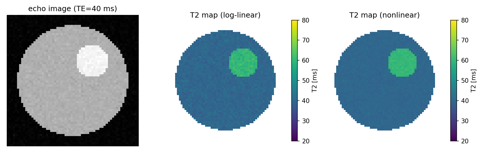
NoteCautions with real data
- Mixed-in fat makes T2 appear longer, so when measuring muscle water T2, use methods that separate fat (multi-component models, fat suppression)
- The first echo is easily affected by “stimulated echoes” from imperfect 180° pulses and is often excluded from the fit
- In magnitude images, noise in the late, near-noise-level echoes does not average to 0 (Rician noise), which makes T2 appear longer
8.5 Python 2: convert a 23Na image to concentration (TSC) with reference phantoms
We build a straight line (calibration curve) from the mean signals of 0 mmol/L (background noise), 20, and 40 mmol/L reference phantoms and convert the whole image to concentration. This is a simplified version of the method used in a skeletal muscle 23Na study (Höger et al. 2023).
code/08_tsc.py
# Convert a 23Na image (synthetic) to tissue sodium concentration TSC [mmol/L] using a reference-phantom calibration line
import numpy as np
import matplotlib.pyplot as plt

rng = np.random.default_rng(3)
N = 96
y, x = np.mgrid[-1:1:N * 1j, -1:1:N * 1j]


def disk(cx, cy, r):
    return (x - cx) ** 2 + (y - cy) ** 2 < r ** 2


# true concentration map [mmol/L]
conc = np.zeros((N, N))
leg = disk(0, -0.1, 0.7)
conc[leg] = 18.0                         # muscle
conc[disk(0.25, -0.25, 0.2) & leg] = 30  # region representing edema
ph20, ph40 = disk(-0.45, 0.78, 0.12), disk(0.45, 0.78, 0.12)
conc[ph20], conc[ph40] = 20.0, 40.0      # reference phantoms
background = disk(0, 0.78, 0.10)         # empty area (0 mmol/L reference)

# acquisition: signal = gain × concentration + offset + noise (gain and offset are unknowns that vary by scanner)
gain, offset = 3.7, 2.0
signal = gain * conc + offset + rng.normal(0, 6.0, conc.shape)

# calibration line: fit a straight line to the mean ROI signals and the known concentrations
known = np.array([0.0, 20.0, 40.0])
measured = np.array([signal[background].mean(), signal[ph20].mean(), signal[ph40].mean()])
a, b = np.polyfit(measured, known, 1)    # concentration = a × signal + b
tsc = a * signal + b
print(f"calibration: TSC = {a:.3f} x signal + {b:.2f}")

muscle_roi = leg & ~disk(0.25, -0.25, 0.25)
edema_roi = disk(0.25, -0.25, 0.15)
print(f"muscle TSC = {tsc[muscle_roi].mean():.1f} mmol/L (true 18)")
print(f"edema  TSC = {tsc[edema_roi].mean():.1f} mmol/L (true 30)")


# two-compartment model: back-calculate the extracellular fluid fraction f_ecw (assuming fixed intracellular fluid f_icw)
def f_ecw_from_tsc(tsc_value, f_icw=0.7, na_ecw=140.0, na_icw=10.0):
    return (tsc_value - f_icw * na_icw) / na_ecw


for name, roi in [("muscle", muscle_roi), ("edema", edema_roi)]:
    print(f"{name}: f_ECW ~ {f_ecw_from_tsc(tsc[roi].mean()):.3f} (assuming f_ICW = 0.7)")

fig, axes = plt.subplots(1, 3, figsize=(12, 3.8))
axes[0].imshow(signal, cmap="gray"); axes[0].set_title("23Na image (a.u.)")
axes[1].plot(measured, known, "o", ms=9, color="#E86A1C")
xs = np.linspace(measured.min(), measured.max(), 10)
axes[1].plot(xs, a * xs + b, color="#3E1485")
axes[1].set(xlabel="mean signal in ROI", ylabel="known [Na+] (mmol/L)", title="calibration line")
h = axes[2].imshow(np.where(leg, tsc, np.nan), cmap="inferno", vmin=0, vmax=40)
axes[2].set_title("TSC map (mmol/L)")
fig.colorbar(h, ax=axes[2], fraction=0.046)
for ax in (axes[0], axes[2]):
    ax.axis("off")
fig.tight_layout()
fig.savefig("figs/08_tsc.png", dpi=150)
calibration: TSC = 0.268 x signal + -0.38
muscle TSC = 18.0 mmol/L (true 18)
edema TSC = 29.8 mmol/L (true 30)
muscle: f_ECW ~ 0.079 (assuming f_ICW = 0.7)
edema: f_ECW ~ 0.163 (assuming f_ICW = 0.7)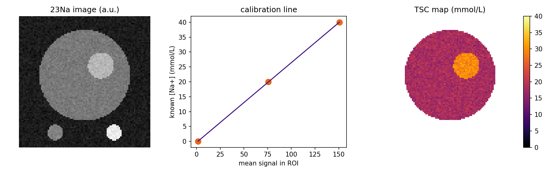
WarningAbout back-calculating with the two-compartment model
This is a calculation built on big assumptions: the intracellular fluid fraction is fixed and the Na concentrations are set to 140 and 10 mmol/L. Rather than trusting the values themselves, use it as a tool to think about “how much of the change in TSC can be explained by changes in extracellular fluid” (Höger et al. 2023).
8.6 Python 3: reading real data (DICOM, NIfTI)
These are templates for reading your own real data (they are not run on this page).
# NIfTI: read the image and the voxel size
import nibabel as nib
import numpy as np

img = nib.load("t2map.nii.gz")
data = img.get_fdata()                    # numpy array (x, y, z)
voxel_mm = img.header.get_zooms()[:3]     # voxel size [mm]
roi = nib.load("roi_gastrocnemius.nii.gz").get_fdata() > 0   # ROI drawn in ITK-SNAP

print("mean T2 in ROI:", data[roi].mean())
print("ROI volume [cm^3]:", roi.sum() * np.prod(voxel_mm) / 1000)
# DICOM: sort a series by TE while checking the acquisition-parameter tags
from pathlib import Path
import numpy as np
import pydicom
files = sorted(Path("dicom_series").glob("*.dcm"))
slices = [pydicom.dcmread(f) for f in files]
slices.sort(key=lambda d: float(d.EchoTime))
te = np.array([float(d.EchoTime) for d in slices]) # [ms]
stack = np.stack([d.pixel_array.astype(float) for d in slices], axis=-1)
print("TE:", te)
print("TR:", slices[0].RepetitionTime, "pixel spacing:", slices[0].PixelSpacing)8.7 Summary
- Original data are DICOM; NIfTI is the standard for research analysis. Convert with dcm2niix
- ROIs with 3D Slicer or ITK-SNAP; brain with FSL and others; MRS with LCModel, jMRUI, and others
- T2 maps come from exponential fitting; TSC comes from a reference-phantom calibration line