flowchart LR
  A["90° pulse<br/>(tip over)"] --> B["Spins dephase<br/>(fast and slow)"]
  B --> C["180° pulse<br/>(flip the arrangement)"]
  C --> D["Fast spins<br/>catch up with slow ones"]
  D --> E["Echo (signal returns)<br/>at time TE"]
2 The NMR Signal and T1/T2
2.1 In a nutshell
- In B0, the body’s magnetization M points along B0 (longitudinal)
- When you apply radio waves at the Larmor frequency (an RF pulse), M is tipped over to the side
- The tipped M rotates and induces an electric current (the signal) in the coil
- Over time, M tries to return to its original longitudinal direction (T1), and its transverse component dephases and disappears (T2)
Because this “way of recovering” and “way of disappearing” differs from tissue to tissue, we can tell tissues apart.
2.2 RF pulses and the flip angle
An RF pulse is a weak magnetic field (B1) oscillating at the Larmor frequency. While B1 is applied, the magnetization is tipped little by little. How far it is tipped is called the flip angle.
- 90° pulse: tips the longitudinal magnetization fully sideways → transverse component is maximal → signal is maximal
- 180° pulse: flips the longitudinal magnetization to the exact opposite (downward) direction (inversion) → used later in Chapter 2 and in the IR method of Chapter 6
2.3 FID: the first signal to appear
The magnetization tipped by a 90° pulse rotates in the transverse plane and induces a voltage in the receive coil. This is the FID (free induction decay). The signal is a wave that “oscillates at the Larmor frequency while gradually getting smaller.”
2.4 T1: the time for longitudinal magnetization to recover (longitudinal relaxation)
The longitudinal component \(M_z\) of the tipped magnetization returns to its original value while handing energy over to its surroundings.
\[ M_z(t) = M_0 \left(1 - e^{-t/T_1}\right) \quad (\text{from right after a 90° pulse}) \]
- T1 is the time to recover to about 63% (\(1 - e^{-1}\)) of the original value
- Fat has a short T1 (recovers quickly); water (such as cerebrospinal fluid) has a long T1 (recovers slowly)
- T1 tends to get longer at higher field strengths
2.5 T2: the time for transverse magnetization to dephase (transverse relaxation)
Right after tipping, many spins rotate in the same direction (in phase), so the signal is large. However, the spins feel each other’s tiny magnetic fields, so their rotation rates gradually drift apart; their directions become scattered and the summed transverse magnetization \(M_{xy}\) gets smaller.
\[ M_{xy}(t) = M_0 \, e^{-t/T_2} \]
- T2 is the time to decay to about 37% (\(e^{-1}\)) of the original value
- Water has a long T2 (for freely moving molecules, the influence of the surroundings averages out). Muscle has a short T2
- When water increases due to edema (swelling, inflammation), muscle T2 becomes longer → used to assess muscle damage after exercise (Höger et al. 2023)
2.6 T2* and the spin echo
In a real scanner, even slight inhomogeneity of the magnetic field itself shifts the spin rotation rates, so the signal disappears faster than T2. This apparent decay time is called T2* (“T2 star”) (T2* ≤ T2).
The shift caused by field inhomogeneity is a “fixed shift,” so if you apply a 180° pulse partway through to flip the arrangement of the spins, the fast and slow spins catch up with each other again and the signal comes back. This is the spin echo (Hahn 1950). Measuring with a spin echo gives the true T2 with the effect of inhomogeneity removed.
2.7 Typical T1 and T2 (3 T, rough values)
| Tissue | T1 (ms) | T2 (ms) | Notes |
|---|---|---|---|
| Skeletal muscle | ~1400 | ~40–50 | Measured at 3 T (Stanisz et al. 2005). In vivo calf muscle: 41–43 ms (Gerhalter et al. 2017; Höger et al. 2023) |
| Fat | ~400 | ~100 | Rough value (wide range depending on source and method) |
| Water (e.g., cerebrospinal fluid) | ~4000 | ~2000 | Rough value |
The demos and code in this material use the rough values above. Real values vary with the scanner, imaging method, and analysis method, so in research either measure them under your own conditions or use literature values obtained under the same conditions.
2.8 Demo: T1 recovery and T2 decay
- Left: fat returns to longitudinal quickly (short T1) → signal is present even when imaging is repeated at short intervals → bright on T1-weighted images
- Right: the transverse signal of water takes a long time to disappear (long T2) → signal remains even when you listen late → bright on T2-weighted images
Choosing between these two properties is the topic of contrast in Chapter 4.
2.9 Python: plot the relaxation curves
code/02_relaxation.py
# Plot T1 recovery and T2 decay curves for each tissue (rough values at 3 T)
import numpy as np
import matplotlib.pyplot as plt

tissues = {  # name: (T1 [ms], T2 [ms], color)
    "fat": (400, 100, "#E86A1C"),
    "muscle": (1400, 45, "#3E1485"),
    "water": (4000, 2000, "#2a76dd"),
}

t1_axis = np.linspace(0, 5000, 500)
t2_axis = np.linspace(0, 300, 500)

fig, (ax1, ax2) = plt.subplots(1, 2, figsize=(10, 3.8))
for name, (T1, T2, c) in tissues.items():
    ax1.plot(t1_axis, 1 - np.exp(-t1_axis / T1), color=c, lw=2.5, label=f"{name} (T1={T1} ms)")
    ax2.plot(t2_axis, np.exp(-t2_axis / T2), color=c, lw=2.5, label=f"{name} (T2={T2} ms)")

ax1.set(title="T1 recovery", xlabel="time [ms]", ylabel="Mz / M0")
ax2.set(title="T2 decay", xlabel="time [ms]", ylabel="Mxy / M0")
for ax in (ax1, ax2):
    ax.legend(frameon=False)
    ax.grid(alpha=0.3)
fig.tight_layout()
fig.savefig("figs/02_relaxation.png", dpi=150)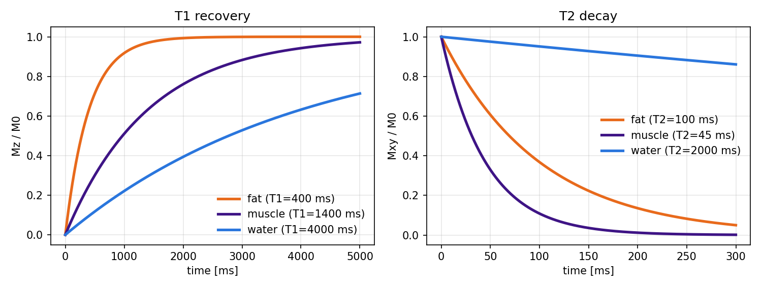
2.10 Summary
- Tipping the magnetization with an RF pulse produces a signal (FID)
- T1: the time for longitudinal magnetization to recover. Short for fat, long for water
- T2: the time for transverse magnetization to dephase and disappear. Long for water, short for muscle. Lengthens with edema
- T2*: the apparent decay including field inhomogeneity. A spin echo can cancel the effect of inhomogeneity