3 Making an Image: Gradients and k-Space
3.1 In a nutshell
The signals up to Chapter 2 are “the sum of signals coming from the whole body,” and we cannot tell where they came from. So we vary the field strength slightly from place to place (gradient fields). Then the rotation frequency changes with position, so looking at the frequency tells us the position (Lauterbur 1973).
3.2 Gradients: turning position into frequency
If the field is made stronger along position \(x\) at a rate of \(G_x\) (mT/m),
\[ f(x) = \frac{\gamma}{2\pi} \left( B_0 + G_x \, x \right) \]
and spins further to the right rotate faster. By splitting the received signal by frequency (the Fourier transform), we can find how much signal there was at each position.
For 1H. For example, with Gx = 10 mT/m, a location 10 cm from the center rotates about 42.6 kHz off.
3.3 The roles of the three gradients
| Role | What it does | In short |
|---|---|---|
| Slice selection | Applies RF while a gradient is on, tipping only a slice of a certain thickness | “Which slice to image” |
| Frequency encoding | Applies a gradient while the signal is being received | Horizontal position → frequency |
| Phase encoding | Applies a brief gradient before reception to shift the rotation angle (phase). Repeated with a different strength each time | Vertical position → phase |
Repeating phase encoding 256 times collects 256 rows of information in the vertical direction. This is why scan time ≈ TR × number of phase-encoding steps × number of averages.
3.4 k-space: the “frequency map” of an image
The collected signals, arranged together, are called k-space. k-space and the image are connected by the 2D Fourier transform.
- Center of k-space: the overall brightness and contrast of the image (slow variations)
- Outer part of k-space: edges and fine details of the image (rapid variations)
3.5 Python: experiencing k-space
We create a simple image mimicking a cross-section of the lower leg (muscle, subcutaneous fat, bone), Fourier-transform it into k-space, and then convert it back into an image keeping only the center or only the outer part.
code/03_kspace.py
# Use a simple lower-leg cross-section phantom to check the roles of the k-space "center" and "edge"
import numpy as np
import matplotlib.pyplot as plt

N = 256
y, x = np.mgrid[-1:1:N * 1j, -1:1:N * 1j]


def disk(cx, cy, r):
    return (x - cx) ** 2 + (y - cy) ** 2 < r ** 2


# Signal intensities (T1-weighted-like: fat is bright)
img = np.zeros((N, N))
img[disk(0, 0, 0.85)] = 1.0    # subcutaneous fat (outer ring)
img[disk(0, 0, 0.75)] = 0.35   # muscle
img[disk(-0.25, -0.2, 0.17)] = 0.05  # cortical bone of the tibia (no signal)
img[disk(-0.25, -0.2, 0.11)] = 0.9   # bone marrow of the tibia (fat)
img[disk(0.35, -0.05, 0.08)] = 0.05  # fibula
img[disk(0.35, -0.05, 0.04)] = 0.9

# image → k-space (2D Fourier transform)
k = np.fft.fftshift(np.fft.fft2(img))

# masks that keep only the k-space center / only the edge
kr = np.hypot(*np.mgrid[-N // 2:N // 2, -N // 2:N // 2])
center = kr < 12
recon_center = np.abs(np.fft.ifft2(np.fft.ifftshift(k * center)))
recon_edge = np.abs(np.fft.ifft2(np.fft.ifftshift(k * ~center)))

fig, axes = plt.subplots(1, 4, figsize=(13, 3.6))
panels = [
    (img, "phantom (image)"),
    (np.log1p(np.abs(k)), "k-space (log |S|)"),
    (recon_center, "only k-space center"),
    (recon_edge, "only k-space edge"),
]
for ax, (im, title) in zip(axes, panels):
    ax.imshow(im, cmap="gray")
    ax.set_title(title)
    ax.axis("off")
fig.tight_layout()
fig.savefig("figs/03_kspace.png", dpi=150)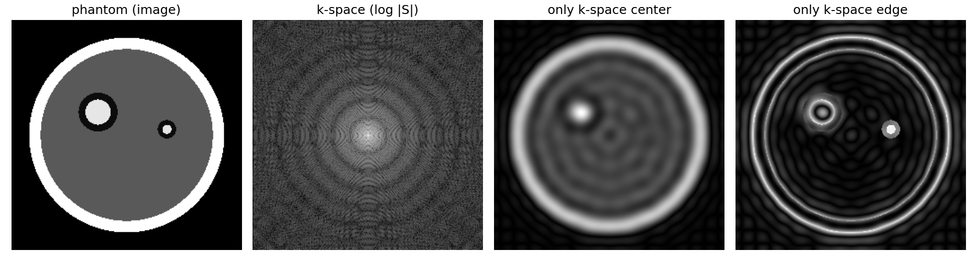
TipLow-resolution 23Na images
Because the 23Na MRI signal is weak, often only the region near the center of k-space can be collected, and the images are blurred like the “only k-space center” panel (e.g., 3 × 3 × 15 mm³ or 4 × 4 × 20 mm³ (Höger et al. 2023)). Therefore, be careful that near muscle boundaries, signal from neighboring tissue gets mixed in (the partial volume effect).
3.6 Summary
- Varying frequency and phase by position with gradients tells us where signal comes from
- The collected signal is k-space; the Fourier transform turns it into an image
- k-space center = contrast, outer part = fine detail