6 Multinuclear MRI: 23Na and 31P
6.1 In a nutshell
Ordinary MRI looks at hydrogen (1H), but by changing the coil and software you can also look at other nuclei.
- 23Na (sodium): the amount of Na outside and inside cells → edema, cell viability, tissue Na accumulation
- 31P (phosphorus): PCr, ATP, inorganic phosphate → muscle energy metabolism, pH
Both have weak signals, so the images are coarse, acquisition takes a long time, and a dedicated coil is required.
6.2 23Na MRI
6.2.1 Characteristics of 23Na
| Property | Details | Consequence |
|---|---|---|
| Low concentration | A few tens of mmol/L in tissue (water hydrogen is ~110 mol/L) | Signal is about 1/10,000 of 1H (Madelin and Regatte 2013) |
| Spin 3/2 | Has a quadrupole moment (electrical asymmetry) and relaxes quickly when interacting with surrounding molecules | Very short T2 (a few ms) |
| Two T2 components | Na with restricted motion shows a short T2 (0.5–5 ms) and a long T2 (10–30 ms) | In calf muscle: short 0.8 ms, long 12.4 ms (Gerhalter et al. 2017) |
| Short T1 | About 30–40 ms in muscle (overall T1 33.8 ms (Gerhalter et al. 2017)) | TR can be shortened to allow many averages |
Because T2 is only a few ms, listening at TE = 10 ms as in ordinary MRI would mean the signal has almost disappeared. Therefore ultra-short TE (UTE, TE ≈ 0.3 ms) acquisitions (such as 3D radial sampling) are used (Höger et al. 2023; Marton et al. 2026).
6.2.2 Na outside and inside cells
| Concentration | Motion | |
|---|---|---|
| Extracellular fluid (interstitial fluid, plasma) | ~140 mmol/L | Moves freely (close to physiological saline) |
| Intracellular fluid | ~10–15 mmol/L | Motion is restricted by collisions with proteins and other molecules |
The outside of the cell is more than 10 times as concentrated because Na⁺/K⁺-ATPase (the sodium pump) pumps Na⁺ out of the cell.
6.2.3 Measure 1: TSC (tissue sodium concentration)
This is the average concentration of all the Na within a voxel (one cell of the image) (mmol/L tissue).
- A reference phantom of known concentration (e.g., tubes of 20 and 40 mmol/L NaCl solidified in agar) is placed beside the leg and imaged together with it, and signal intensity is converted to concentration (Höger et al. 2023; Marton et al. 2026) (code implemented in Chapter 8)
- Muscle TSC is about 10–25 mmol/L depending on the study (e.g., tibialis anterior 11.7 and gastrocnemius 14.3 mmol/L (Höger et al. 2023); calf muscles 22–25 mmol/L (Marton et al. 2026)). Values change with the imaging, calibration, and analysis methods, so be careful when comparing absolute values across studies
6.2.3.1 Two-compartment model
TSC can be thought of as the volume-weighted average of extracellular and intracellular Na.
\[ TSC \approx f_{ECW} \times 140 + f_{ICW} \times 10 \quad [\text{mmol/L}] \]
(\(f_{ECW}\), \(f_{ICW}\): volume fractions of extracellular and intracellular fluid in the voxel. The solid fraction is treated as 0)
Because extracellular Na is 14 times more concentrated, even a small increase in extracellular fluid raises TSC substantially. In one example, the rise in TSC in participants whose muscles swelled after exercise could be largely explained by extracellular edema using this model (Höger et al. 2023).
The fraction values are assumptions for illustration. For example, just changing f_ECW from 0.10 to 0.15 raises TSC by 7 mmol/L.
6.2.4 Measure 2: ICwS (intracellular-weighted sodium signal) = the IR method
This is the same idea as STIR in Chapter 5. After inverting with a 180° pulse and waiting TI,
\[ M_z(TI) = M_0 \left(1 - 2 e^{-TI/T_1}\right), \qquad TI_{\text{null}} = T_1 \ln 2 \]
Freely moving Na (extracellular fluid, edema, blood) has a longer T1, and Na with restricted motion (intracellular) has a shorter T1, so imaging at the TI where free Na becomes 0 leaves the more intracellular Na (Nagel et al. 2011).
- Example: TI = 34 ms (Höger et al. 2023) → the component with \(T_1 = 34 / \ln 2 \approx 49\) ms becomes 0 (a setting that nulls saline-like Na)
- Separation is not complete and extracellular components are also mixed in, so it is called intracellular-weighted (Höger et al. 2023)
The two T1 values are assumptions for illustration. With TI around 35 ms, free Na (orange) is almost 0 and only restricted Na (purple) gives signal (signal magnitude is the absolute value of Mz).
6.2.5 Measure 3: TQF (triple-quantum filter)
This method uses a phenomenon specific to spin-3/2 Na (the quadrupolar interaction) to selectively measure only Na whose motion is restricted by binding to macromolecules. It is mainly interpreted as more intracellular, but it also includes Na interacting with interstitial macromolecules (Gerhalter et al. 2017). Because the signal is even weaker, it is often measured as a spectrum (Chapter 7) rather than an image.
6.2.6 What is it used for?
- Exercise and muscle damage: TSC and ICwS rise right after eccentric exercise and return to baseline by 48 hours (whereas water T1 and T2 rise at 48 hours) (Höger et al. 2023)
- Rapid changes in extracellular fluid: when calf blood volume was changed with a cuff, the 23Na measures changed more sensitively than 1H T2 (Gerhalter et al. 2017)
- Hypertension and aldosteronism: muscle Na accumulation was measured and shown to decrease with KCl supplementation (Marton et al. 2026)
- Elevated intracellular Na in muscle channelopathies and muscular dystrophies (Nagel et al. 2011)
6.3 31P MRS
6.3.1 What 31P shows
31P is almost always measured as a spectrum (signal arranged by frequency) rather than an image (MRS, Chapter 7). Each phosphorus-containing molecule has a different chemical shift (ppm), so the peaks appear separated. Taking PCr as 0 ppm,
| Peak | Position (ppm, approx.) | Meaning |
|---|---|---|
| Pi (inorganic phosphate) | ~+4.9 (moves with pH) | Product after ATP is used. Its position gives intracellular pH |
| PCr (phosphocreatine) | 0 (reference) | An energy reserve for quickly regenerating ATP |
| γ-ATP | ~−2.5 | The terminal one of ATP’s three phosphates |
| α-ATP | ~−7.5 | |
| β-ATP | ~−16 | Comes only from ATP, so used to quantify ATP |
In resting skeletal muscle, PCr has been reported at around 30 mmol/L and ATP at around 8 mmol/L (per intracellular water; varies by source) (Kemp et al. 2007).
6.3.2 How to obtain pH
The ratio of Pi’s two forms (H₂PO₄⁻ and HPO₄²⁻) changes with pH, and the peak appears at their averaged position. Therefore intracellular pH can be calculated from the distance δ (ppm) between PCr and Pi (Moon and Richards 1973). One commonly used formula:
\[ pH = 6.75 + \log_{10} \frac{\delta - 3.27}{5.63 - \delta} \]
6.3.3 Exercise and recovery: assessing mitochondrial capacity
- During exercise: PCr is broken down to replenish ATP, so PCr↓ and Pi↑ (pH may also drop)
- After exercise: mitochondria produce ATP, and PCr recovers exponentially
\[ PCr(t) = PCr_{end} + \left(PCr_{rest} - PCr_{end}\right)\left(1 - e^{-t/\tau}\right) \]
The shorter the recovery time constant τ (PCr recovery time constant), the higher the mitochondrial oxidative capacity, according to the usual interpretation. Recommendations for measurement and analysis are summarized in an expert consensus paper (Meyerspeer et al. 2020).
6.3.4 Python: 31P spectrum and PCr recovery
code/06_p31.py
# Compute pH from a (synthetic) 31P spectrum and estimate the time constant τ from post-exercise PCr recovery
import numpy as np
import matplotlib.pyplot as plt
from scipy.optimize import curve_fit

rng = np.random.default_rng(1)


def lorentz(ppm, center, amp, width=0.3):
    return amp * (width / 2) ** 2 / ((ppm - center) ** 2 + (width / 2) ** 2)


# --- 1. synthetic spectrum (peak positions and heights are rough values for illustration) ---
ppm = np.linspace(-20, 10, 3000)
peaks = {"Pi": (4.90, 0.15), "PCr": (0.0, 1.0), "g-ATP": (-2.5, 0.25),
         "a-ATP": (-7.5, 0.25), "b-ATP": (-16.2, 0.22)}
spec = sum(lorentz(ppm, c, a) for c, a in peaks.values())
spec += rng.normal(0, 0.01, ppm.size)

# find the Pi peak position and compute pH
mask = (ppm > 3.5) & (ppm < 6.0)
delta = ppm[mask][np.argmax(spec[mask])]
pH = 6.75 + np.log10((delta - 3.27) / (5.63 - delta))
print(f"Pi - PCr shift = {delta:.2f} ppm -> pH = {pH:.2f}")

# --- 2. estimate τ from post-exercise PCr recovery (synthetic data) ---
t = np.arange(0, 300, 6.0)                 # every 6 s for 5 min [s]
true_tau = 35.0
pcr = 0.55 + (1.0 - 0.55) * (1 - np.exp(-t / true_tau))
pcr_obs = pcr + rng.normal(0, 0.02, t.size)


def recovery(t, pcr_end, pcr_rest, tau):
    return pcr_end + (pcr_rest - pcr_end) * (1 - np.exp(-t / tau))


popt, pcov = curve_fit(recovery, t, pcr_obs, p0=(0.5, 1.0, 30))
tau, tau_se = popt[2], np.sqrt(pcov[2, 2])
print(f"PCr recovery tau = {tau:.1f} +/- {tau_se:.1f} s (true {true_tau} s)")

fig, (ax1, ax2) = plt.subplots(1, 2, figsize=(11, 3.8))
ax1.plot(ppm, spec, color="#3E1485")
for name, (c, a) in peaks.items():
    ax1.annotate(name, (c, a + 0.04), ha="center")
ax1.invert_xaxis()                          # NMR convention: ppm decreases to the right
ax1.set(xlabel="chemical shift [ppm] (PCr = 0)", ylabel="signal", title="31P spectrum (synthetic)")
ax2.plot(t, pcr_obs, "o", color="#999", label="measured")
ax2.plot(t, recovery(t, *popt), color="#E86A1C", lw=2.5, label=f"fit: tau = {tau:.0f} s")
ax2.set(xlabel="time after exercise [s]", ylabel="PCr / PCr_rest", title="PCr recovery")
ax2.legend(frameon=False)
fig.tight_layout()
fig.savefig("figs/06_p31.png", dpi=150)
Pi - PCr shift = 4.88 ppm -> pH = 7.08
PCr recovery tau = 36.5 +/- 2.1 s (true 35.0 s)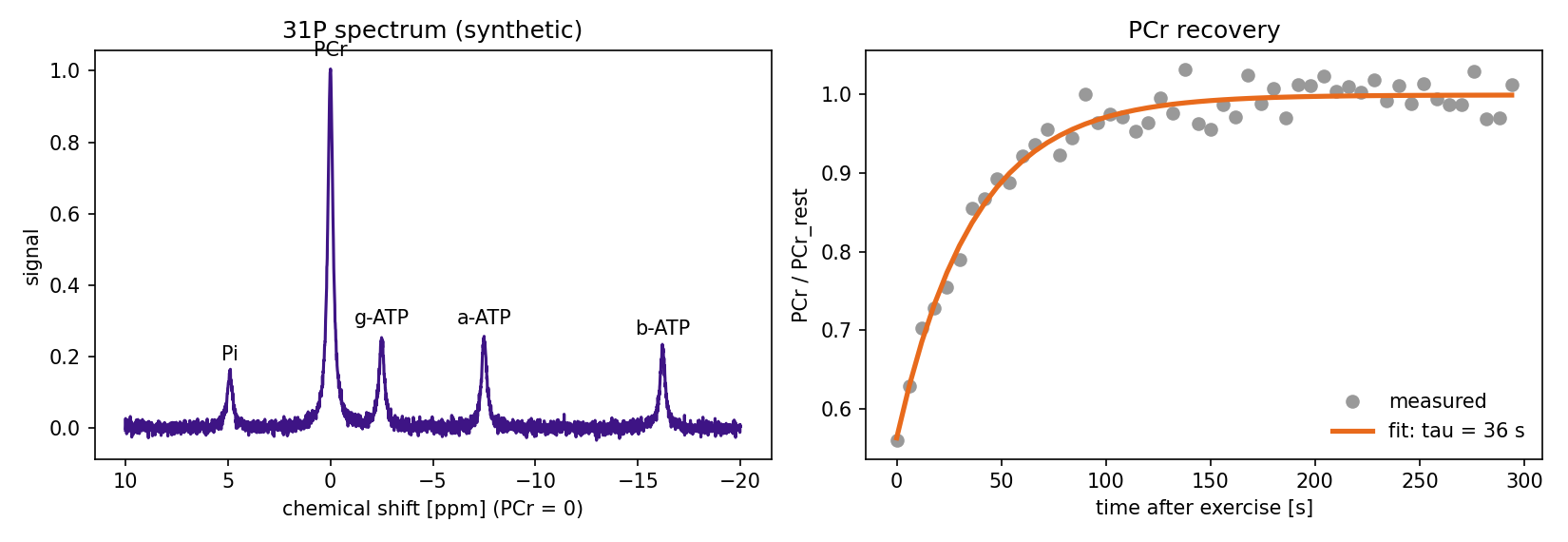
6.4 Other nuclei
- 13C: its natural abundance is low (1.1%), so it is used to measure glycogen in muscle and liver, and to observe metabolism with “hyperpolarization,” which uses special equipment to boost the signal tens of thousands of times
- 19F: almost absent from the body, so only fluorine-containing drugs and contrast agents appear clearly
- 39K: intracellular K⁺. Sensitivity is extremely low, so it is for research at ultra-high field (7 T and above)
6.5 Summary
- 23Na: T2 is short (a few ms), so ultra-short TE is required. TSC (total Na), ICwS (intracellular-weighted, with free Na nulled by IR), TQF (restricted Na)
- TSC is very sensitive to changes in extracellular fluid (two-compartment model). Absolute values depend on imaging and calibration methods
- 31P: spectra of PCr, ATP, and Pi. pH from the Pi position; mitochondrial capacity from the post-exercise PCr recovery τ