5 Separating Fat and Muscle
5.1 In a nutshell
Fat and water (muscle) both give hydrogen signals. There are two main clues for separating them.
- Difference in T1: fat has a short T1 → bright on T1-weighted images, and inversion recovery (STIR) can null fat alone
- A slight difference in rotation frequency (chemical shift): fat hydrogen rotates about 3.4 ppm slower than water hydrogen → suppress fat by selecting its frequency (fat suppression), or separate them by their phase difference (the Dixon method)
5.2 Chemical shift: the same hydrogen has a different frequency depending on surrounding electrons
A hydrogen nucleus is slightly protected (shielded) by the electrons around it, so the magnetic field it feels is a little weaker. Water (H₂O) and fat (rich in –CH₂–) have different electron environments, so the main fat peak rotates at a frequency about 3.4 ppm lower than water (ppm = parts per million).
\[ \Delta f = 3.4 \times 10^{-6} \times f_0 \approx 434 \ \text{Hz} \quad (3\ \text{T},\ f_0 = 127.7\ \text{MHz}) \]
At 1.5 T it is about 217 Hz. We exploit this frequency difference.
5.3 Method 1: look at and trace T1-weighted images
This is the simplest method. On T1-weighted images fat is bright and muscle is gray, so you separate the fat and muscle regions manually or by thresholding and measure their area (cross-sectional area, CSA) or volume. However, when fat is finely mixed into the muscle (fatty infiltration), a single pixel contains both and becomes an ambiguous gray that is neither.
5.4 Method 2: fat suppression (frequency-selective)
Using an RF pulse tuned only to the fat frequency (water −434 Hz), you first tip and null only the fat magnetization and then image (the CHESS method, “Fat Sat”). Its weakness is that field inhomogeneity shifts the frequency, which tends to make suppression non-uniform.
5.5 Method 3: STIR (nulling fat with inversion recovery)
After inverting all the longitudinal magnetization with a 180° pulse, if you wait for a time TI, it recovers as
\[ M_z(TI) = M_0 \left(1 - 2 e^{-TI/T_1}\right) \]
If you image exactly at the moment when \(M_z = 0\), that tissue gives no signal.
\[ TI_{\text{null}} = T_1 \ln 2 \approx 0.69 \, T_1 \]
For fat (T1 ≈ 400 ms), TI ≈ 280 ms. In an actual lower-leg study, a T2-weighted STIR-type sequence (TIRM) with TI = 260 ms was used to observe edema (Höger et al. 2023). Applying the same idea to 23Na gives the IR (intracellular-weighted) method in Chapter 6.
5.6 Method 4: the Dixon method (splitting into water and fat images)
Because water and fat rotate at rates that differ by 434 Hz (3 T), as time passes they alternate between pointing the same way (in-phase, IP) and pointing opposite ways (opposed-phase, OP) (Dixon 1984).
- in-phase: \(S_{IP} = W + F\)
- opposed-phase: \(S_{OP} = W - F\)
From these two images,
\[ W = \frac{S_{IP} + S_{OP}}{2}, \qquad F = \frac{S_{IP} - S_{OP}}{2}, \qquad FF = \frac{F}{W + F} \]
we can create a water image, a fat image, and a fat fraction map. At 3 T, opposed-phase is at TE ≈ 1.15 ms and in-phase at TE ≈ 2.3 ms (\(1/(2\Delta f)\) and \(1/\Delta f\)).
Note“PDFF” as used in research
Real fat has multiple peaks and is also affected by T2* and T1. The fat fraction that corrects for these and is precisely defined as a ratio of amounts of hydrogen is called PDFF (proton density fat fraction), and it is standard to measure it with multi-echo (around 6 echoes) Dixon methods (Reeder et al. 2012; Hu and Kan 2013). It is widely used to assess liver fat and intramuscular fat in muscle diseases and aging.
5.7 Demo: water and fat signals reinforce and cancel depending on TE
Set the fat fraction to 0.5 and the signal becomes almost 0 at opposed-phase (water and fat cancel each other completely).
5.8 Python: create water, fat, and fat fraction maps with 2-point Dixon
We create a lower-leg phantom with fatty infiltration (FF 15%) in part of the muscle and separate it from in-phase / opposed-phase images. Finally, we use the fat fraction to measure the cross-sectional areas of muscle and subcutaneous fat.
code/05_dixon.py
# 2-point Dixon method: obtain water image, fat image, and fat fraction from in-phase / opposed-phase
import numpy as np
import matplotlib.pyplot as plt

rng = np.random.default_rng(0)
N = 200
fov_cm = 12.0                      # field of view 12 cm → 0.06 cm per pixel
pix_area = (fov_cm / N) ** 2       # [cm^2]
y, x = np.mgrid[-1:1:N * 1j, -1:1:N * 1j]


def disk(cx, cy, r):
    return (x - cx) ** 2 + (y - cy) ** 2 < r ** 2


# true water amount W and fat amount F (relative values)
W = np.zeros((N, N))
F = np.zeros((N, N))
F[disk(0, 0, 0.9)] = 0.95; W[disk(0, 0, 0.9)] = 0.05     # subcutaneous fat
W[disk(0, 0, 0.78)] = 0.80; F[disk(0, 0, 0.78)] = 0.0     # muscle
infil = disk(0.25, 0.35, 0.22) & disk(0, 0, 0.78)
W[infil] = 0.68; F[infil] = 0.12                          # fatty infiltration (FF 15%)
bone = disk(-0.3, -0.2, 0.16)
W[bone] = 0.0; F[bone] = 0.0                              # cortical bone
marrow = disk(-0.3, -0.2, 0.10)
F[marrow] = 0.9; W[marrow] = 0.05                         # bone marrow

# acquisition: IP = W + F, OP = W - F (complex in reality; here an ideal case with no phase error)
noise = 0.01
S_ip = W + F + rng.normal(0, noise, W.shape)
S_op = W - F + rng.normal(0, noise, W.shape)

# separation
W_est = (S_ip + S_op) / 2
F_est = (S_ip - S_op) / 2
signal = W_est + F_est
FF = np.where(signal > 0.1, F_est / np.maximum(signal, 1e-6), np.nan)

# classify by fat fraction (FF < 0.5 = muscle, FF >= 0.5 = fat). Exclude the tibia region to leave out bone marrow
tissue = signal > 0.1
muscle = tissue & (FF < 0.5)
fat = tissue & (FF >= 0.5) & ~disk(-0.3, -0.2, 0.16)
print(f"muscle CSA = {muscle.sum() * pix_area:.1f} cm^2")
print(f"fat CSA    = {fat.sum() * pix_area:.1f} cm^2")
print(f"mean FF in infiltrated region = {np.nanmean(FF[infil]) * 100:.1f} %")

fig, axes = plt.subplots(1, 5, figsize=(15, 3.4))
for ax, (im, title, kw) in zip(axes, [
    (S_ip, "in-phase", {}), (S_op, "opposed-phase", {}),
    (W_est, "water", {}), (F_est, "fat", {}),
    (FF, "fat fraction", {"vmin": 0, "vmax": 1, "cmap": "magma"}),
]):
    h = ax.imshow(im, cmap=kw.pop("cmap", "gray"), **kw)
    ax.set_title(title)
    ax.axis("off")
fig.colorbar(h, ax=axes[-1], fraction=0.046)
fig.tight_layout()
fig.savefig("figs/05_dixon.png", dpi=150)
muscle CSA = 65.2 cm^2
fat CSA = 22.6 cm^2
mean FF in infiltrated region = 15.0 %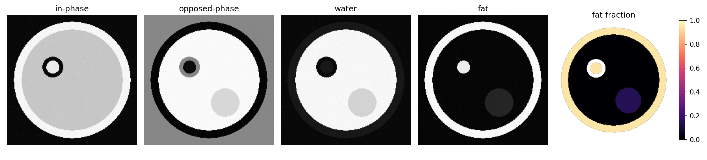
WarningPitfalls of 2-point Dixon
Real signals are complex-valued and carry phase shifts due to field inhomogeneity. If you compute using only the magnitude (absolute value), there will be places where you cannot tell whether water or fat dominates (a W–F swap). Product Dixon methods (mDixon, IDEAL, etc.) solve this with phase correction and multiple echoes. The code above is “an explanation of the principle under ideal conditions.”
5.9 Which method should you use?
| Purpose | Commonly used method |
|---|---|
| Cross-sectional area or volume of muscle and fat (shape) | T1-weighted or Dixon water/fat images → segmentation |
| Amount of fat within muscle (quality) | Multi-echo Dixon PDFF |
| Looking at edema or inflammation | Fat-suppressed T2-weighted, STIR, water T2 map (with the effect of fat removed) |
| T1, T2, and fat fraction all at once | MR fingerprinting (Ma et al. 2013) |
5.10 Summary
- Fat and water can be separated by the difference in T1 and the difference in frequency (chemical shift of 3.4 ppm)
- STIR nulls fat with TI = T1 × ln2
- Dixon creates water images, fat images, and fat fraction from in-phase / opposed-phase. In research, multi-echo Dixon PDFF is the standard