# Exercises {#sec-exercises}
```{r}
#| echo: false
source("R/setup.R")
```
Let's try what we have covered so far on new data. The solutions are collapsed. **Write your own code first**, then open them.
## Data: children's dental growth (`Orthodont`)
This dataset is from the nlme package (included with R by default). For 27 children (16 boys, 11 girls), the distance (mm) from the pituitary to the pterygomaxillary fissure was measured at ages 8, 10, 12, and 14.
```{r}
data(Orthodont, package = "nlme")
ortho <- as.data.frame(Orthodont)
ortho$Subject <- factor(as.character(ortho$Subject))
head(ortho)
```
- `distance`: distance (mm) ← response variable
- `age`: age (8, 10, 12, 14)
- `Subject`: child ID ← group
- `Sex`: sex (Male / Female)
## Exercise 1: Visualization
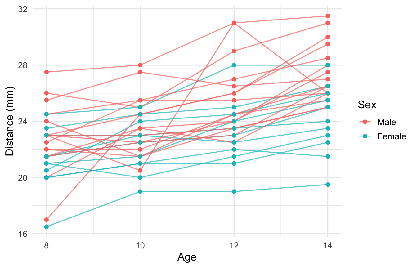
Draw the relationship between `age` and `distance` for each child as a line, colored by sex. What trends do you see?
::: {.callout-tip collapse="true"}
## Example solution
```{r}
ggplot(ortho, aes(age, distance, group = Subject, colour = Sex)) +
  geom_line(alpha = 0.7) + geom_point() +
  labs(x = "Age", y = "Distance (mm)")
```
- Distance increases with age
- The starting level differs by child (a random intercept seems necessary)
- Boys seem larger overall, and seem to grow more
:::
## Exercise 2: Random-intercept model
Fit a model that adds a by-child random intercept to `distance ~ age`, and find
(a) the amount of growth per year
(b) the variation between children (SD) and the residual SD
(c) the ICC
::: {.callout-tip collapse="true"}
## Example solution
```{r}
m1 <- lmer(distance ~ age + (1 | Subject), data = ortho)
summary(m1)
vc <- as.data.frame(VarCorr(m1))
icc <- vc$vcov[1] / sum(vc$vcov)
icc
```
(a) Growth of about `r round(fixef(m1)["age"], 2)` mm per year
(b) Between-child SD ≈ `r round(vc$sdcor[1], 2)`, residual SD ≈ `r round(vc$sdcor[2], 2)`
(c) ICC ≈ `r round(icc, 2)`. Most of the variation is due to differences between children
:::
## Exercise 3: Centering age
The intercept of the model in Exercise 2 is "the distance at age 0", which is outside the range of the data and cannot be interpreted.
Create a variable `age8` by subtracting 8 from `age`, and refit the model so that the intercept is "the average distance at age 8". Does the slope estimate change?
::: {.callout-tip collapse="true"}
## Example solution
```{r}
ortho$age8 <- ortho$age - 8
m1c <- lmer(distance ~ age8 + (1 | Subject), data = ortho)
rbind(Original = fixef(m1), Centered = fixef(m1c))
```
The slope does not change; only the intercept changes to "the value at age 8".
:::
## Exercise 4: Random-slope model
Fit a model `m2` in which the slope of `age8` also varies by child, and compare it with the model `m1c` from Exercise 3. Is the random slope needed?
::: {.callout-tip collapse="true"}
## Example solution
```{r}
m2 <- lmer(distance ~ age8 + (age8 | Subject), data = ortho)
VarCorr(m2)
anova(m1c, m2, refit = FALSE)
```
The fixed effects are the same, so we compare with REML as is (`refit = FALSE`).
Decide by looking at the p-value and AIC. If the p-value is around 0.05, also take into account that
the p-value is conservative because of the boundary problem (Chapter @sec-inference). In this data, individual differences in the slope are fairly small,
and the conclusions about the fixed effects hardly change whichever model you choose.
:::
## Exercise 5: Effect of sex
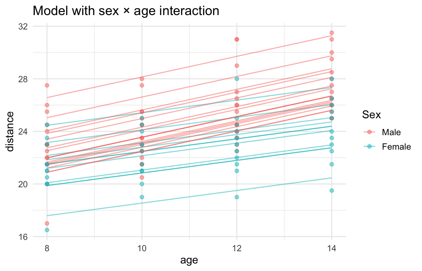
Let's examine whether there is a sex difference in how children grow.
(a) Create a model `m3` that adds `Sex` and `age8:Sex` (the interaction) as fixed effects (the random effect `(1 | Subject)` is fine)
(b) Compare it with the model without the interaction, `m3a`, using a likelihood ratio test
(c) Explain the results in words
::: {.callout-tip collapse="true"}
## Example solution
```{r}
m3  <- lmer(distance ~ age8 * Sex + (1 | Subject), data = ortho)
m3a <- lmer(distance ~ age8 + Sex + (1 | Subject), data = ortho)
summary(m3)$coefficients
anova(m3a, m3) # fixed effects differ, so the models are refitted with ML
```
(c) The reference category is `Male` (check with `levels(ortho$Sex)`).
- `(Intercept)`: average distance for boys at age 8
- `age8`: growth per year for boys
- `SexFemale`: difference girls − boys at age 8
- `age8:SexFemale`: difference in growth rate (girls − boys). If negative, girls grow more slowly
If the p-value of the likelihood ratio test is small, we can say that "there is a sex difference in growth rate".
```{r}
ortho$pred <- predict(m3)
ggplot(ortho, aes(age, distance, colour = Sex)) +
  geom_point(alpha = 0.5) +
  geom_line(aes(y = pred, group = Subject), alpha = 0.5) +
  labs(title = "Model with sex × age interaction")
```
:::
## Exercise 6: Diagnostics
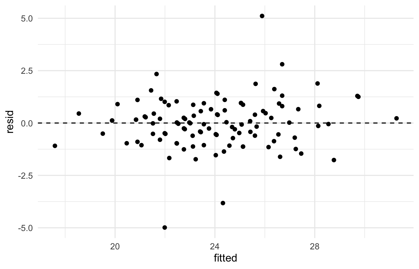
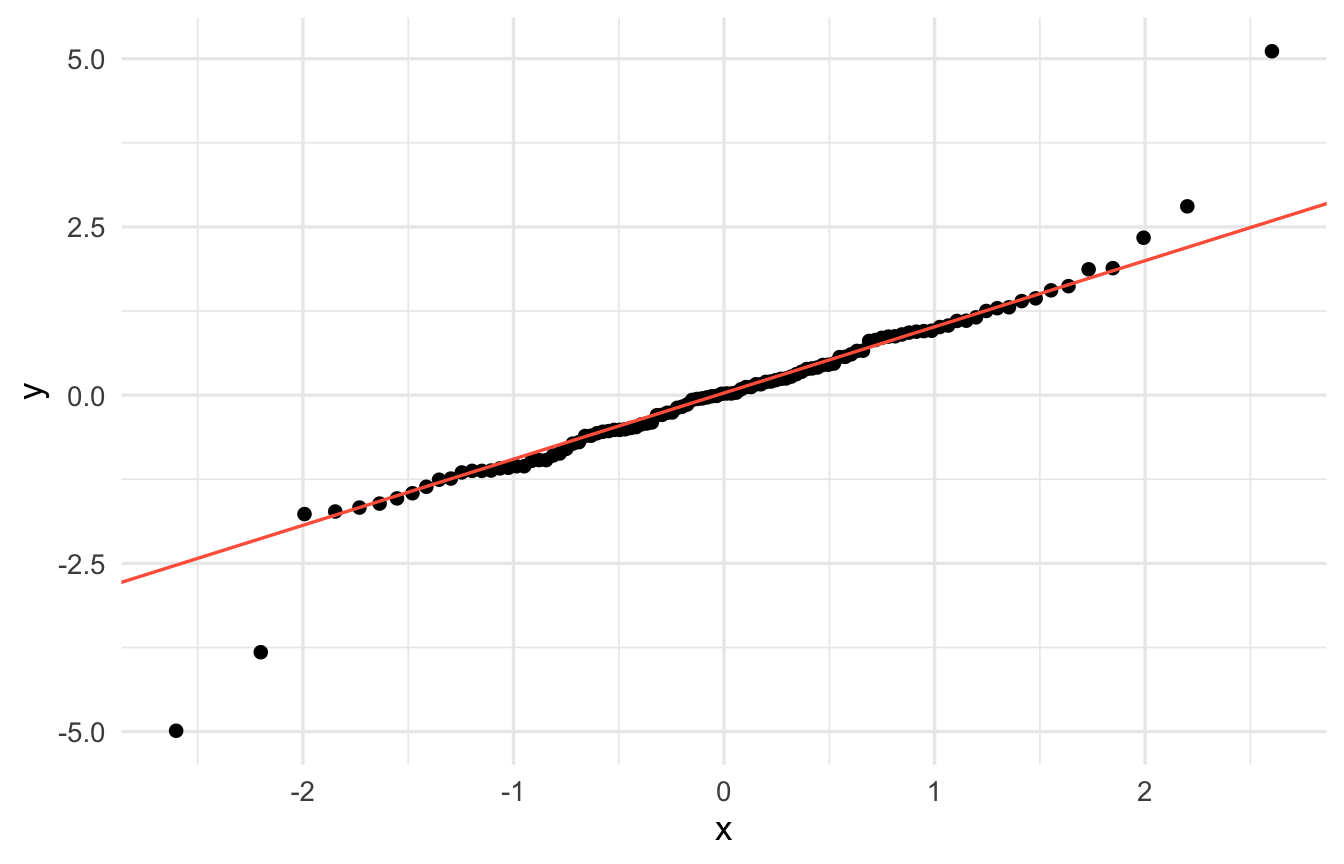
For the model `m3` from Exercise 5, draw a residuals vs fitted plot and a Q-Q plot of the residuals, and check whether there are any problems.
::: {.callout-tip collapse="true"}
## Example solution
```{r}
dd <- data.frame(fitted = fitted(m3), resid = resid(m3), Subject = ortho$Subject)

ggplot(dd, aes(fitted, resid)) +
  geom_point() + geom_hline(yintercept = 0, linetype = 2)
ggplot(dd, aes(sample = resid)) + stat_qq() + stat_qq_line(colour = "tomato")
# check the observations with the largest residuals
ortho[order(-abs(resid(m3)))[1:4], c("Subject", "age", "distance", "Sex")]
```
In this data, measurements of some children (e.g., M09, M13) show fairly large residuals.
It is a good idea to consider whether they may be outliers, and to check whether the conclusions change when they are removed (sensitivity analysis).
:::
## Advanced exercises
1. In the simulation in Chapter @sec-why, what happens to the false positive rate of `lmer` if you reduce the number of schools from 20 to 6? (A caution for when there are few groups)
2. Modify `sim_school()` to create data in which the slope also differs by school, and check whether a random-slope model can recover the true values.
3. In `sleepstudy`, try analyzing `Days` 0–1 (the training period) separately from day 2 onward (in fact, sleep restriction in this data starts from day 2).
Well done!