# Diagnostics and reporting {#sec-diagnostics}
```{r}
#| echo: false
source("R/setup.R")
data(sleepstudy)
fit_rs <- lmer(Reaction ~ Days + (Days | Subject), data = sleepstudy)
```
## Checking the model assumptions
The main assumptions of a linear mixed model are:
1. The fixed-effects part is **linear**
2. The residuals $\varepsilon_{ij}$ are normally distributed with constant variance
3. The random effects $u_j$ are normally distributed
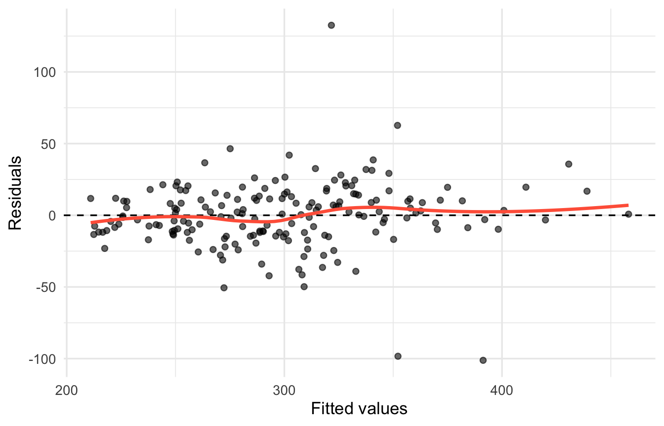
### Residuals vs fitted values
```{r}
diag_df <- data.frame(fitted = fitted(fit_rs), resid = resid(fit_rs))

ggplot(diag_df, aes(fitted, resid)) +
  geom_point(alpha = 0.6) +
  geom_hline(yintercept = 0, linetype = 2) +
  geom_smooth(se = FALSE, colour = "tomato") +
  labs(x = "Fitted values", y = "Residuals")
```
- OK if the residuals are scattered **evenly** around 0
- Funnel shape (spreading out to the right) → the variance is not constant. Consider transforming the response, e.g., taking logs
- A curved pattern → the relationship is not linear. Consider adding a quadratic term, etc.
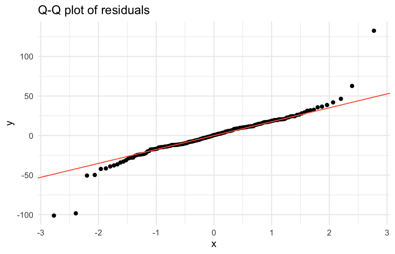
### Normal Q-Q plot of the residuals
```{r}
ggplot(diag_df, aes(sample = resid)) +
  stat_qq() + stat_qq_line(colour = "tomato") +
  labs(title = "Q-Q plot of residuals")
```
If the points lie roughly on a straight line, the normality assumption is reasonable. It is common for the ends to deviate a little.
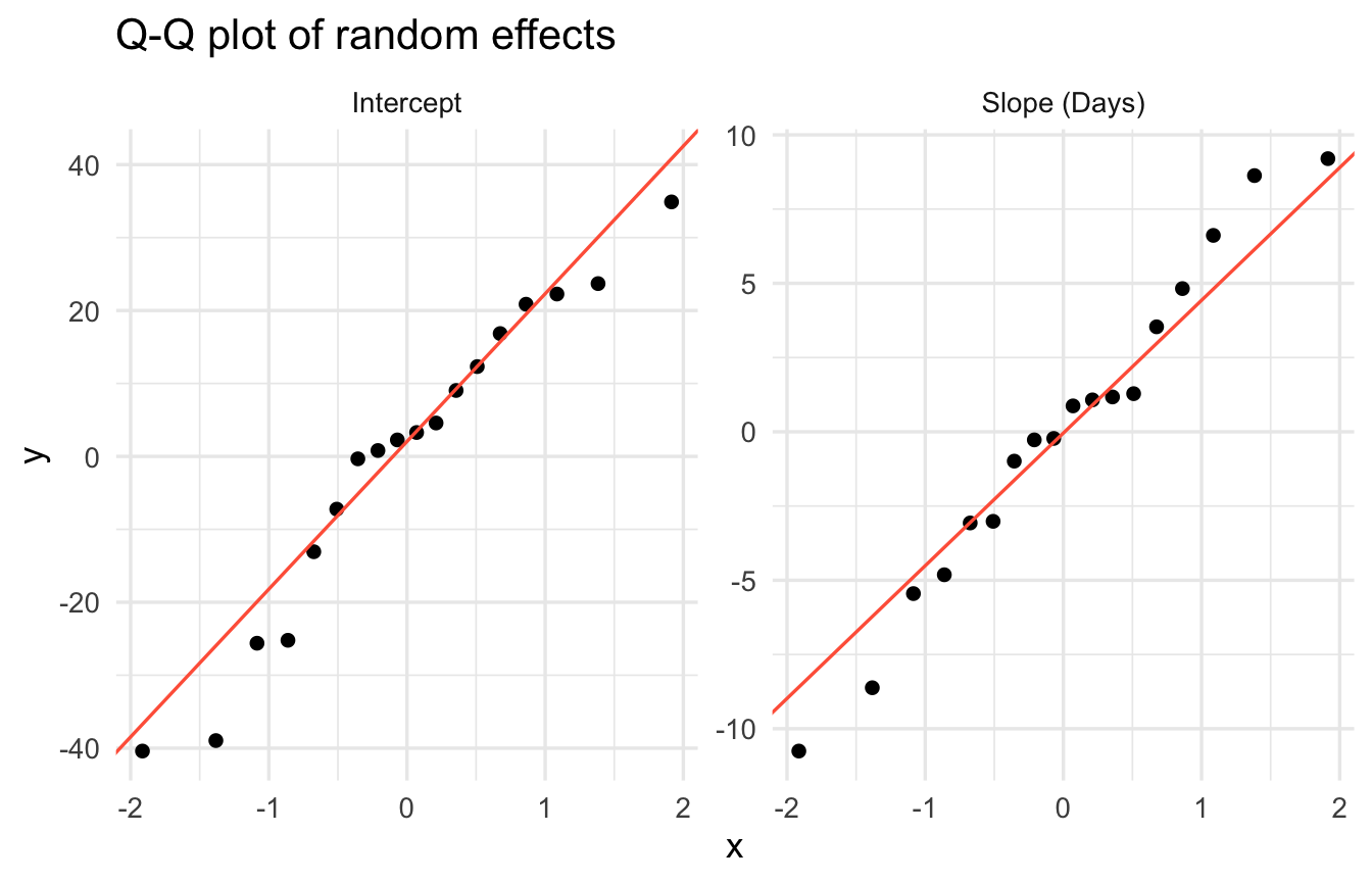
### Q-Q plot of the random effects
```{r}
re <- ranef(fit_rs)$Subject
re_long <- data.frame(value = c(re[, 1], re[, 2]),
                      term  = rep(c("Intercept", "Slope (Days)"), each = nrow(re)))

ggplot(re_long, aes(sample = value)) +
  stat_qq() + stat_qq_line(colour = "tomato") +
  facet_wrap(~ term, scales = "free") +
  labs(title = "Q-Q plot of random effects")
```
With few groups (here, 18 people) it is hard to judge, but check that there are no extreme outliers.
::: {.callout-tip}
With `check_model(fit)` from the **performance** package, you can draw all these diagnostic plots at once (`install.packages("performance")`).
:::
## Common warnings and how to deal with them
### `boundary (singular) fit: see help('isSingular')`
This appears when a random-effect variance is **estimated as 0**, or a correlation is estimated as ±1.
```{r}
#| warning: true
#| message: true
set.seed(3)
g <- factor(rep(1:10, each = 5))
x <- runif(50)
y <- 1 + 2 * x + rnorm(50)          # data with actually no group differences
fit_sing <- lmer(y ~ x + (1 | g))
VarCorr(fit_sing)
isSingular(fit_sing)
```
Main causes and remedies:
- There really is almost no variation between groups → drop that random effect (the results are almost the same without it)
- The random-effects structure is too complex for the data → simplify `(x | g)` to `(x || g)` or `(1 | g)`
- Too few groups
### `Model failed to converge`
This appears when the optimization (the search for parameters) does not converge properly.
- **Put the predictors on a similar scale** (centering / standardizing): e.g., `scale(x)`
- Change the optimization algorithm: `lmer(..., control = lmerControl(optimizer = "bobyqa"))`
- Try multiple algorithms with `allFit(fit)` and check whether the results agree
- Simplify the random-effects structure
::: {.callout-note}
## Centering is recommended
The intercept is "the value when all predictors are 0". For variables where 0 is not meaningful, such as age or height,
subtracting the mean (`x_c = x - mean(x)`) makes the intercept "the value at an average x", which is easier to interpret,
and it also reduces the correlation between intercept and slope, which stabilizes estimation.
:::
## Reporting the results
In a paper or report, include at least the following information.
1. **Model structure**: response variable, fixed effects, random effects, groups
2. **Estimation method and software**: REML / ML, versions of R and lme4, how p-values were computed
3. **Fixed effects**: estimates, standard errors (or 95% confidence intervals), test results
4. **Random effects**: each SD (or variance), correlations
```{r}
ci <- confint(fit_rs, parm = "beta_", method = "Wald")
fe <- summary(fit_rs)$coefficients
vc <- as.data.frame(VarCorr(fit_rs))

fe_tab <- data.frame(
  Estimate = round(fe[, "Estimate"], 2),
  SE     = round(fe[, "Std. Error"], 2),
  `95%CI` = sprintf("[%.2f, %.2f]", ci[, 1], ci[, 2]),
  df     = round(fe[, "df"], 1),
  t      = round(fe[, "t value"], 2),
  p      = format.pval(fe[, "Pr(>|t|)"], digits = 2, eps = 0.001),
  check.names = FALSE
)
knitr::kable(fe_tab, caption = "Fixed effects")
knitr::kable(
  data.frame(Group = vc$grp, Term = ifelse(is.na(vc$var2), vc$var1, paste(vc$var1, "×", vc$var2)),
             `SD / Corr` = round(vc$sdcor, 2), check.names = FALSE),
  caption = "Random effects"
)
```
### Example report text
> A linear mixed model with reaction time as the response, days of sleep restriction as a fixed effect, and by-participant random intercepts and random slopes for days (with their correlation) was fitted by REML using the lme4 package (`r packageVersion("lme4")`) in R (`r getRversion()`). Fixed effects were tested using the Satterthwaite approximation from the lmerTest package.
> Reaction time increased on average by `r sprintf("%.1f", fe["Days", "Estimate"])` ms per day of sleep restriction (95% CI [`r sprintf("%.1f", ci["Days", 1])`, `r sprintf("%.1f", ci["Days", 2])`], *t*(`r sprintf("%.1f", fe["Days", "df"])`) = `r sprintf("%.2f", fe["Days", "t value"])`, *p* < .001). The SD of individual differences in the slope was `r sprintf("%.1f", vc$sdcor[2])` ms/day.
## Next steps
- **Generalized linear mixed models (GLMMs)**: for when the response is 0/1 (pass/fail) or a count. E.g., `lme4::glmer(y ~ x + (1 | g), family = binomial)`
- **Bayesian estimation**: the `brms` package. Converges more easily even for complex models, and lets you handle uncertainty directly
- **Further reading**
- Takuya Kubo, *Introduction to Statistical Modeling for Data Analysis* (Iwanami Shoten; in Japanese) — from GLMs to GLMMs and Bayesian methods
- Gelman & Hill "Data Analysis Using Regression and Multilevel/Hierarchical Models"
- Bates et al. (2015) "Fitting Linear Mixed-Effects Models Using lme4", *Journal of Statistical Software* 67(1)
::: {.callout-important}
## Chapter summary
- Check the assumptions with residual plots and Q-Q plots
- Singular fit → consider simplifying the random effects. No convergence → rescale variables or change the optimizer
- When reporting, write "model structure, estimation method, fixed effects, random effects" as a set
:::